Estimating Oculus Rift pixel density

A few months ago I bought an Oculus Rift DK2. Although these are designed for VR gaming, they’re actually pretty reasonable stereo displays. They have several desirable features, particularly that the OLED display is pulsed stroboscopically each frame to reduce motion blur. However, this also means that each pixel is updated at the same time, unlike on most LCD panels, meaning they can be used for timing sensitive applications. As of a recent update they are also supported by Psychtoolbox, which we use to run the majority of experiments in the lab. Lastly, they’re reasonably cheap, at about £300.

In starting to set up an experiment using the goggles I thought to check what their effective pixel resolution was in degrees of visual angle. Because the screens are a fixed distance from the wearer’s eye, I (foolishly) assumed that this would be a widely available value. Quite a few people simply took the monocular resolution (1080 x 1200) and divided this by the nominal field of view (110° vertically), producing an estimate of about 10.9 pixels per degree. As it turns out, this is pretty much bang on, but that wasn’t necessarily the case, because the lenses produce increasing levels of geometric distortion (bowing) at more eccentric locations. This might have the effect of concentrating more pixels in the centre of the display, increasing the number of pixels per degree.

Anyway, I decided it was worth verifying these figures myself. Taking a cue from methods we use to calibrate mirror stereoscopes, here’s what I did…

First I created two calibration images, consisting of a black background, and either one central square, or two lateralised squares. All the squares were 200 pixels wide (though this isn’t crucial), and the one with two squares was generated at the native resolution of the Oculus Rift (2160×1200). Here’s how the first one looks:

And here’s how the other one, with only one square looked:

These images were created with a few lines of Matlab code:

ORw = 2160; % full width of the oculus rift in pixels
ORh = 1200; % height of the oculus rift in pixels
CSw = 1440; % height of other computer's display in pixels
CSh = 900;  % width of other computer's display in pixels
ORs = 200;  % width of the squares shown on the rift
CSs = 200;  % width of the square shown on the computer's display

a = zeros(ORh,ORw);
a((1+ORh/2-ORs/2):(ORh/2+ORs/2),(1+ORw/4-ORs/2):(ORw/4+ORs/2)) = 1;
a((1+ORh/2-ORs/2):(ORh/2+ORs/2),(1+3*ORw/4-ORs/2):(3*ORw/4+ORs/2)) = 1;
imwrite(a,'ORimage.jpg','jpeg')

a = zeros(CSh,CSw);
a((1+CSh/2-CSs/2):(CSh/2+CSs/2),(1+CSw/2-CSs/2):(CSw/2+CSs/2)) = 1;
imwrite(a,'CSimage.jpg','jpeg')

I then plugged in the Rift, and displayed the two-square image on it, and the one-square image on an iPad (though in principle this could be any screen, or even a printout). Viewed through the Rift, each square goes to only one eye, and the binocular percept is of a single central square.

Now comes the clever bit. The rationale behind this method is that we match the perceived size of a square shown on the Rift with one shown on the iPad. We do this by holding the goggles up to one eye, with the other eye looking at the iPad. It’s necessary to do this at a bit of an angle, so the square gets rotated to be a diamond, but we can rotate the iPad too to match the orientation. I found it pretty straightforward to get the sizes equal by moving the iPad forwards and backwards, and using the pinch-to-zoom operation.

Once the squares appeared equal in size I put the Rift down, but kept the iPad position fixed. I then measured two things: the distance from the iPad to my eye, and the width of the square on the iPad screen. The rest is just basic maths:

The iPad square was 7.5cm wide, and matched the Rift square at 24cm from the eye. At that distance an object 1cm wide subtends 2.4° of visual angle (because at 57cm, 1cm=1°). [Note, for the uninitiated, the idea of degrees of visual angle is that you imagine a circle that goes all the way around your head, parallel to your eyes. You can divide this circle into 360 degrees, and each individual degree will be about the size of a thumbnail held at arm’s length. The reason people use this unit is that it can be calculated for a display at any distance, allowing straightforward comparison of experimental conditions across labs.] That means the square is 2.4*7.5=18° wide. Because this is matched with the square on the Rift, the Rift square is also 18° wide. We know the square on the Rift is 200 pixels wide, so that means 18° = 200 pix, and 1° = 11 pixels. So, the original estimates were correct, and the pixel density at the centre of the screen is indeed 11 pixels/deg.

This is actually quite a low resolution, which isn’t surprising since the screen is close to the eye, individual pixels are easily visible, and the whole point of the Rift is to provide a wide field of view rather than a high central resolution. But it’s sufficient for some applications, and its small size makes it a much more portable stereo display than either a 3D monitor or a stereoscope. I’m also pleased I was able to independently verify other people’s resolution estimates, and have developed a neat method for checking the resolution of displays that aren’t as physically accessible as normal monitors.

Aesthetically pleasing, publication quality plots in R

I spend a lot of my time making graphs. For a long time I used a Unix package called Grace. This had several advantages, including the ability to create grids of plots very easily. However it also had plenty of limitations, and because it is GUI-based, one had to create each plot from scratch. Although I use Matlab for most data analysis, I’ve always found its plotting capabilities disappointing, so a couple of years ago I bit the bullet and started learning R, using the RStudio interface.

There are several plotting packages for R, including things like ggplot2, which can automate the creation of some plots. Provided your data are in the correct format, this can make plotting really quick, and tends to produce decent results. However, for publication purposes I usually want to have more control over the precise appearance of a graph. So, I’ve found it most useful to construct graphs using the ‘plot’ command, but customising almost every aspect of the graph. There were several things that took me a while to work out, as many functions aren’t as well documented as they could be. So I thought it would be helpful to share my efforts. Below is some code (which you can also download here) that demonstrates several useful techniques for plotting, and should create something resembling the following plot when executed.

Example plot created by the script.

My intention is to use this script myself as a reminder of how to do different things (at the moment I always have to search through dozens of old scripts to find the last time I did something), and copy and paste chunks of code into new scripts each time I need to make a graph. Please feel free to use parts of it yourself, to help make the world a more beautiful place!

# this script contains examples of the following:
# outputting plots as pdf and eps files
# creating plots with custom tick mark positioning
# drawing points, bars, lines, errorbars, polygons, legends and text (including symbols)
# colour ramps, transparency, random numbers and density plots

# Code to output figures as either an eps or pdf file. Note that R’s eps files appear not to cope well with transparency, whereas pdfs are fine
outputplot <- 0
if(outputplot==1){postscript(“filename.eps”, horizontal = FALSE, onefile = FALSE, paper = “special”, height = 4.5, width = 4.5)}
if(outputplot==2){pdf(“filename.pdf”, bg=”transparent”, height = 5.5, width = 5.5)}
# all the code to create the plot goes here
if(outputplot>0){dev.off()}  # this line goes after you’ve finished plotting (to output the example below, move it to the bottom of the script)

# set up an empty plot with user-specified axis labels and tick marks
plotlims <- c(0,1,0,1)  # define the x and y limits of the plot (minx,maxx,miny,maxy)
ticklocsx <- (0:4)/4    # locations of tick marks on x axis
ticklocsy <- (0:5)/5    # locations of tick marks on y axis
ticklabelsx <- c(“0″,”0.25″,”0.5″,”0.75″,”1”)        # set labels for x ticks
ticklabelsy <- c(“0″,”0.2″,”0.4″,”0.6″,”0.8″,”1”)    # set labels for y ticks

par(pty=”s”)  # make axis square
plot(x=NULL,y=NULL,axes=FALSE, ann=FALSE, xlim=plotlims[1:2], ylim=plotlims[3:4])   # create an empty axis of the correct dimensions
axis(1, at=ticklocsx, tck=0.01, lab=F, lwd=2)     # plot tick marks (no labels)
axis(2, at=ticklocsy, tck=0.01, lab=F, lwd=2)
axis(3, at=ticklocsx, tck=0.01, lab=F, lwd=2)
axis(4, at=ticklocsy, tck=0.01, lab=F, lwd=2)
mtext(text = ticklabelsx, side = 1, at=ticklocsx)     # add the tick labels
mtext(text = ticklabelsy, side = 2, at=ticklocsy, line=0.2, las=1)  # the ‘line’ command moves away from the axis, the ‘las’ command rotates to vertical
box(lwd=2)      # draw a box around the graph
title(xlab=”X axis title”, col.lab=rgb(0,0,0), line=1.2, cex.lab=1.5)    # titles for axes
title(ylab=”Y axis title”, col.lab=rgb(0,0,0), line=1.5, cex.lab=1.5)

# create some synthetic data to plot as points and lines
datax <- sort(runif(10,min=0,max=1))
datay <- sort(runif(10,min=0.2,max=0.8))
SEdata <- runif(10,min=0,max=0.1)
lines(datax,datay, col=’red’, lwd=3, cex=0.5)     # draw a line connecting the points
arrows(datax,datay,x1=datax, y1=datay-SEdata, length=0.015, angle=90, lwd=2, col=’black’)  # add lower error bar
arrows(datax,datay,x1=datax, y1=datay+SEdata, length=0.015, angle=90, lwd=2, col=’black’)  # add upper error bar
points(datax,datay, pch = 21, col=’black’, bg=’cornflowerblue’, cex=1.6, lwd=3)   # draw the data points themselves

# create some more synthetic data to plot as bars
datax <- 0.1*(1:10)
datay <- runif(10,min=0,max=0.2)
SEdata <- runif(10,min=0,max=0.05)
ramp <- colorRamp(c(“indianred2”, “cornflowerblue”))  # create a ramp from one colour to another
colmatrix <- rgb(ramp(seq(0, 1, length = 10)), max = 255)   # index the ramp at ten points
barplot(datay, width=0.1, col=colmatrix, space=0, xlim=1, add=TRUE, axes=FALSE, ann=FALSE)  # add some bars to an existing plot
arrows(datax-0.05,datay,x1=datax-0.05, y1=datay-SEdata, length=0.015, angle=90, lwd=2, col=’black’)  # add lower error bar
arrows(datax-0.05,datay,x1=datax-0.05, y1=datay+SEdata, length=0.015, angle=90, lwd=2, col=’black’)  # add upper error bar

coltrans=rgb(1,0.5,0,alpha=0.3)             # create a semi-transparent colour (transparency is the alpha parameter, from 0-1)
a <- density(rnorm(100,mean=0.75,sd=0.1))   # make a density distribution from some random numbers
a$y <- 0.2*(a$y/max(a$y))                   # rescale the y values for plotting
polygon(a$x, 1-a$y, col=coltrans,border=NA) # plot upside down hanging from the top axis with our transparent colour

# create a legend that can contain lines, points, or both
legend(0, 1, c(“Lines”,”Points”,”Both”), cex=1, col=c(“darkgrey”,”black”,”black”), pt.cex=c(0,1.8,1.8), pt.bg=c(“black”,”violet”,”darkgreen”),lty=c(1,0,1), lwd=c(5,3,3), pch=21, pt.lwd=3, box.lwd=2)
# add text somewhere, featuring symbols and formatting
text(0.8,0.95,substitute(paste(italic(alpha), ” = 1″ )),cex=1.2,adj=0)

In Rainbows

Our department recently obtained a custom-made Psychology logo rainbow flag to celebrate pride month.

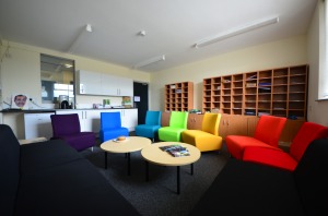
This matches the rainbow seating in our staff room!

Vision in amblyopia

In recent years there have been a number of treatments proposed for amblyopia in adults. These treatments (reviewed in this paper) often involve balancing the inputs to the two eyes – down-weighting the input to the stronger eye to allow the weaker eye to contribute. The treatments improve visual function in the amblyopic eye, and some patients have even recovered stereo vision (e.g. see this TEDx video by ‘stereo’ Sue Barry). However we know very little about the mechanisms by which these improvements occur, or indeed what the nature of the neural deficits in amblyopia actually are.

Today a new paper came out online in the journal Investigative Ophthalmology & Vision Science. In it, we show that neural responses in amblyopia are reduced in the affected eye. We used a steady-state visual evoked potential technique to measure responses in each eye. The reductions are large enough that they could potentially be used to monitor improvements in visual function during treatment.

These data served as the pilot results for a grant proposal that was recently funded by the Centre for Chronic Diseases and Disorders (and part-funded by the Wellcome Trust). The plan is to use both fMRI and EEG to understand the architecture of the amblyopic binocular visual system, and to monitor improvements in visual function during a course of therapy. A postdoc job is available for 18 months to work on this project, and I’d be very interested in hearing from qualified applicants before the deadline (27th February 2015).

Welcome to new PhD students

Our term started last week. Returning to the lab is Greta Vilidaitė. Greta completed a summer project last year, and now returns as a PhD student. Her project will investigate abnormalities of neural noise in autism spectrum disorders. She is pictured here drinking some very strong mead from her native Lithuania.

Another new addition is Dave Coggan. Dave completed our Cognitive Neuroscience masters course last year, and now returns to start a PhD supervised by Tim Andrews and myself. He will study processes of mid-level vision using fMRI. He is pictured here singing at the annual ECR karaoke night.

Conferences and various things

I’ve just finished a very busy term. It was my first term of proper teaching, which took up a lot more time than I was expecting. It seemed to go well though – I got some very positive feedback from the students, as well as some hilarious comments (“Iron your shirts!!!” being my favourite…).

I’ve also been planning two conferences that we’re holding at York this year. The AVA meeting is in a few weeks time on the 11th April. We’ve got some excellent talks lined up, and have just finalised the program. Also, the BACN meeting is taking place in September, so still plenty of time to submit abstracts for that.

Last week I was up in Glasgow, where I gave a talk in the optometry department at Glasgow Caledonian. I also went to an excellent gig at King Tut’s Wah Wah Hut, where my old band played a few times about 15 years ago. We saw two bands from the 90s: Republica and Space. It looked like this:

Space at King Tut’s

Other than that, I’ve had a couple of papers out this year, and am working on some more. I’m also anxiously awaiting news of a BBSRC grant proposal I put in back in September. I got some very positive reviews in January, and should hear next month whether it’s been funded. Fingers crossed!

Arduino sound to TTL trigger for EEG

A recent query on the Psychtoolbox mailing list about triggers for EEG prompted me to write an explanation of the system we developed at York to do this. I use the method below for steady state EEG, but it should work just as well for ERP designs. The arduino sound trigger was first constructed by my colleague Becky Gilbert, and she has kindly allowed me to share the design and her code.

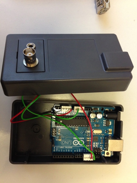
It uses an Arduino UNO, to which we attached an audio jack socket to the analog input pin A0 (and a ground pin), and a BNC socket to the digital output pin 13. The board was mounted in a standard box. We had our technician drill holes in the box and mount the ports in it for stability. The whole thing is small (11×6.5cm), and powered from USB. Here is a picture with the lid off:

 

We then used the arduino software to upload a script to the board (appended below). It’s a very simple bit of code that just monitors the analog input for changes in voltage above a specific threshold. When a voltage change happens it sends a brief trigger on the digital output, at the appropriate voltage for a TTL pulse. Note that on some systems this pulse is too brief to be detected. If this occurs, inserting a brief pause (e.g. uncomment the //delay(100);) after the digitalWrite(outPin, HIGH) line will extend the pulse.

I connect the jack socket to the headphone socket of the stimulus computer, and the BNC to the trigger socket on the EEG/MEG amplifier system. I use the PsychPortAudio commands in Psychtoolbox to produce a 50ms binary pulse:

PsychPortAudio(‘FillBuffer’, tr, ones(1,220));

which I play at stimulus onset (e.g. directly after a Flip command) using:

PsychPortAudio(‘Start’, tr);

I’ve tested the arduino with an oscilloscope, and it responds within a millisecond of receiving the sound pulse. Of course, the timing accuracy of the sound pulse will depend on your computer hardware – see the PTB documentation and use PsychPortAudioTimingTest to check this. On most systems I’ve tried, the latency is very small indeed, so triggers should be completed well within one screen refresh.

I hope people find this useful, and particular credit to Becky (@BeckyAGilbert) for designing the system. If you have any problems, please leave comments below. Of course producing the box requires a some soldering, and we take no responsibility for any resulting injury, death etc. 😉

 

 

#define DEBUG 0 // change to 1 to debug 
 
 #define THRESHOLD 0.1 // adjust this to control sensitivity in detection of voltage increase
 
 const int outPin = 13; // change output (D) pin number here
 int prev_voltage = 0; // must be initialized to something
 
 void setup() {
  if(DEBUG) {
   // initialize serial communication at 9600 bits per second (to write debugging info back to terminal)
    Serial.begin(9600); 
  }
  // set output pin
  pinMode(outPin, OUTPUT);
  
 }
 
 void loop() {
   // read input on analog pin 0
  int sensorValue = analogRead(A0); // change input (A) pin number here
  // convert analog reading (from 0-1023) to digital
  float voltage = sensorValue * (5.0 / 1023.0);
 
 if(DEBUG) {
    // print value to serial port (view in Tools > Serial Port Monitor)
    Serial.println(voltage); // This delays the trigger by
                             // about 6ms so remove before using
                             // during experiments
 }
    // Simplest algorithm ever.  
    if (voltage > prev_voltage + THRESHOLD)
    {
      digitalWrite(outPin, HIGH);
//delay(100);
    }
    else
    {
     digitalWrite(outPin, LOW); 
    }
    
   prev_voltage = voltage;
 }

Videos of ECVP noise symposium

A few weeks ago, at ECVP in Bremen, we held a symposium entitled “Visual noise: new insights”. The talks were varied and interesting, and have been recorded for the benefit of those who were unable to attend the symposium.

The videos are available via the following YouTube links:

Introduction
Remy Allard
Stan Klein [Slides (with additional notes)]
Josh Solomon
Peter Neri
Keith May
Daniel Baker [Slides]
Discussion

Details of the talks (including abstracts) are available here.

Many thanks to Udo Ernst and his team for hosting and filming the event, and Keith May for editing and uploading the videos.

On learning new motor skills

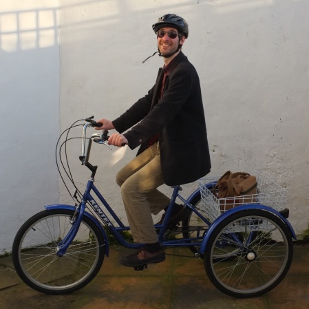
About four weeks ago, at the age of 31, I learned to ride a bike. This followed some six months of travelling around by tricycle:

Me on my tricycle

Although the trike is great, and really useful for transporting shopping and other things around in its basket, sometimes it just doesn’t go very fast. Also, drunk guys walking home from the pub find it hilarious – as do my friends:

Especially Mladen…

So anyway, last month I finally consented to undergo cycling lessons. Mostly, this involved a couple of hours in a car park after work trying to get both feet on the pedals without falling off. Eventually I managed, and then progressed to some advanced techniques, like using the gears and going round corners.

The interesting bit about learning to ride as an adult was how counterintuitive balancing on a bike turns out to be. If you feel like you’re about to topple off to the left, instinct says you should lean or steer to the right. That’s what you’d do if you were balancing on a beam or something. But on a bike, you do the opposite. Falling to the left is fixed by steering and leaning leftwards.

Apparently this is to do with physics. Imagine going round a corner on a bike. You lean into the curve, which causes the bike to accelerate round the bend (probably this is centrifugal force, but high school physics was a long time ago – it may have changed since then…). If you did the opposite, the whole thing would topple over. I found a nice explanation of some of this here.

Physics aside, the amazing thing is how quickly learning this counterintuitive rule becomes automatic. In fact, now I’ve got the hang of it, I don’t even know I’m doing it. Since most people learn to cycle as children, it must seem so much like second nature that they can’t understand how anyone wouldn’t be able to do it. Also, I definitely felt like I got better in my sleep, which is apparently pretty standard for consolidating motor skills.

I got quite excited about learning to ride, so I went and bought a shiny new bike. Then last week did a 46k ride with some friends from work. I was surprised how much fun that was, and somehow ended up agreeing to do the Action Medical Research York 100k bike ride that took place yesterday. Coincidentally, it left from right outside the psychology department – the very place I’d learned to cycle a few weeks before!

The ride was mostly enjoyable, with a few tough hills, and lots of wind on the last leg. We had good weather though, and managed to get round all 100km (actually more like 106) in 6 hours 45 minutes. I feel much more confident after cycling all that way… Here’s a photo at the finish line:

Tess, Mark and I just after finishing.

Why can some people’s brains see better than others’?

On Friday I had a new paper published in the open access journal PLoS ONE. It addresses the question of why some people have better sensitivity to contrast (variations in light levels across an image) than others, sometimes by quite substantial amounts. Unlike differences in eyesight (acuity) that can usually be optically corrected, contrast sensitivity differences occur even for large (low frequency) stimuli that aren’t affected much by optical blur. Presumably then, the sensitivity differences are neural in origin. I was surprised that nobody had really tried to answer this question before, so thought I should give it a go.

The paper is divided into two parts. The first section uses an equivalent noise technique to assess whether sensitivity differences are due to different amounts of noise, or a difference in the efficiency with which stimuli are processed. Although I rule out the latter explanation, the noise masking method cannot tease apart a difference in internal noise from a difference in contrast gain. So, the second part of the study looks at a large corpus of contrast discrimination data, collated from 18 studies in the literature. By looking at the between-subject differences in discrimination performance, I conclude that individual differences at threshold are primarily a consequence of differences in contrast gain. Whether this is due to differences in structure, anatomy, neurotransmitter levels or developmental factors is unclear at the moment.

Since I spent quite a long time putting together all of the dipper function data, I thought I should make it available online. Most of the data were extracted from the published figures using the excellent GraphClick program. The data can be downloaded here in Matlab format. They are organised into a cell array, with each of the 22 cells containing data from one experiment. Each cell is further divided into separate cells for each individual observer, with the ‘data’ array containing the x- and y-values used to produce these plots. I hope these data become a useful resource for other researchers interested in basic visual processes.